CPTAC ccRCC: paired global proteomics

Know what was prepared upstream

Input scope of the prepared CPTAC example. Protein-to-gene mapping, filtering and paired modelling take place upstream of lisaR.

The supplied primary table has 6,482 usable, unique gene-symbol rows for the 80-pair comparison. Its declared effect is tumor_minus_nat, so a positive value means higher tumour abundance. The ranking column is the moderated limma t from the upstream paired model. p_value and fdr_bh_all_genes remain in the table. lisaR uses the full ranked table and does not refit limma or pre-filter genes by significance for this route.

Protein measurements were mapped to gene identifiers and filtered before this input was exported. The useful coverage for this example is therefore the number of usable mapped gene rows, not a count of all originally measured protein features. The frozen input audit records zero duplicate Entrez IDs, zero missing Entrez IDs and zero non-finite values in the required numeric columns. It does not establish the total number of protein features before mapping, how many-to-one mappings were resolved or how many features were discarded at each filter. A mapping percentage or protein-level coverage claim cannot be recovered from 6,482 gene rows alone.

The global proteomic profile configures warnings below 500 usable features and below 1,500 usable features. These are operational warning thresholds, not validated scientific minima. A targeted panel has a limited feature universe and needs its own coverage assessment; it is not represented by this global-proteomic example. Tumour tissue and adjacent tissue also differ in cellular composition, which this prepared differential-abundance table does not resolve.

Use a short writable project root. The examples below use D:/lisa on Windows; change the drive if needed. Avoid nesting the project under several long folder names. Preparation creates study.yml, short inputs under data/ and a provenance/path_map.tsv linking them to their original names and hashes. Results go to out/. Scientific comparison names and directions are unchanged.

1. Obtain the reviewed bundle

Install lisaR first with Installation, then make the external membership resource available through Resources and provenance. Obtain the reviewed input bundle in a new destination:

library(lisaR)
root <- if (.Platform$OS.type == "windows") "D:/lisa" else "~/lisa"
root <- path.expand(root)
dir.create(file.path(root, "bundles"), recursive = TRUE, showWarnings = FALSE)

bundle <- install_lisa_example_bundle(
  "cptac-ccrcc",
  destination = file.path(root, "bundles", "cptac")
)
bundle$next_command

The default source is a versioned public release in DBM-OlmedaLab/lisaR-example-data. The installer verifies the pinned archive and the six-file member manifest before promoting it. A verified cached archive can be reused offline. The bundle contains the primary table and five audit files, but acquiring it does not run lisaR.

bundle$next_command is a complete POSIX shell command with prepare-only mode enabled. To prepare from R or RStudio using the current R installation:

2. Create and check the prepared project

project <- normalizePath(file.path(root, "cptac"),
                         winslash = "/", mustWork = FALSE)
Sys.setenv(
  LISAR_CPTAC_CCRCC_BUNDLE = bundle$bundle,
  LISAR_CPTAC_CCRCC_PROJECT_DIR = project,
  LISAR_CPTAC_CCRCC_PREPARE_ONLY = "1"
)
prepare_script <- system.file("examples", "cptac-ccrcc",
  "prepare_and_run_cptac_ccrcc.R", package = "lisaR")
status <- system2(file.path(R.home("bin"), "Rscript"),
                  c("--vanilla", shQuote(prepare_script)))
Sys.unsetenv("LISAR_CPTAC_CCRCC_PREPARE_ONLY")
stopifnot(status == 0L)

Preparation verifies and copies the inputs, resolves resources, validates and plans the project, then reports CPTAC_CCRCC_LOCAL_ROUTE=PREPARE_ONLY_PASS. It performs no new differential-abundance fit and does not call run_lisa(). The promoted directory is an execution-ready prepared project, not a completed scientific result.

3. Inspect the configuration and its output plan

config <- file.path(project, "study.yml")
study <- yaml::read_yaml(config)
print(study$pipeline)
print(data.frame(
  analysis = study$single_de[[1]]$analysis_id,
  comparison = study$single_de[[1]]$comparison,
  positive_direction = study$single_de[[1]]$positive_direction,
  rank_column = study$single_de[[1]]$rank_col
))
validation <- validate_lisa_config(config, check_files = TRUE)
stopifnot(validation$execution_ready)
output_plan <- plan_lisa_outputs(config)
print(output_plan$summary)

This inspection and plan_lisa_outputs() describe the intended products. They do not execute GSEA. Check that the analysis is cptac_ccrcc_tumor_minus_nat, the effect direction is tumour minus NAT and the ranking column is t before proceeding.

4. Run, verify and recognise the result

result <- run_lisa(config)
check <- verify_lisa_run(result$output_dir)
stopifnot(identical(result$gate, "PASS"), identical(check$gate, "PASS"))
print(result$output_dir)
browseURL(file.path(result$output_dir, "report_index.html"))

The generated configuration has one DE analysis, cptac_ccrcc_tumor_minus_nat, and no LISA profile contrast in this example. It uses global proteomic, one worker, the four semantic collections and the resource identities lisa_dictionary_core@1.0.0, msigdb_term2gene@2026.1 and lisa_category_map@1.0.0. Hallmarks, ORA and native KEGG maps are disabled. This is a choice for the example, not a restriction on proteomic studies in lisaR.

A successful run is written to project/out. Verification must report gate PASS. In the report, positive NES follows the prepared tumour-minus-NAT ranking. No responder grouping, healthy-donor comparison or protein-level model has been added by lisaR.

STANDARD provides category plots and linked gene-set/gene evidence. The report guide shows how to add selected presentation products to a completed run without repeating enrichment.

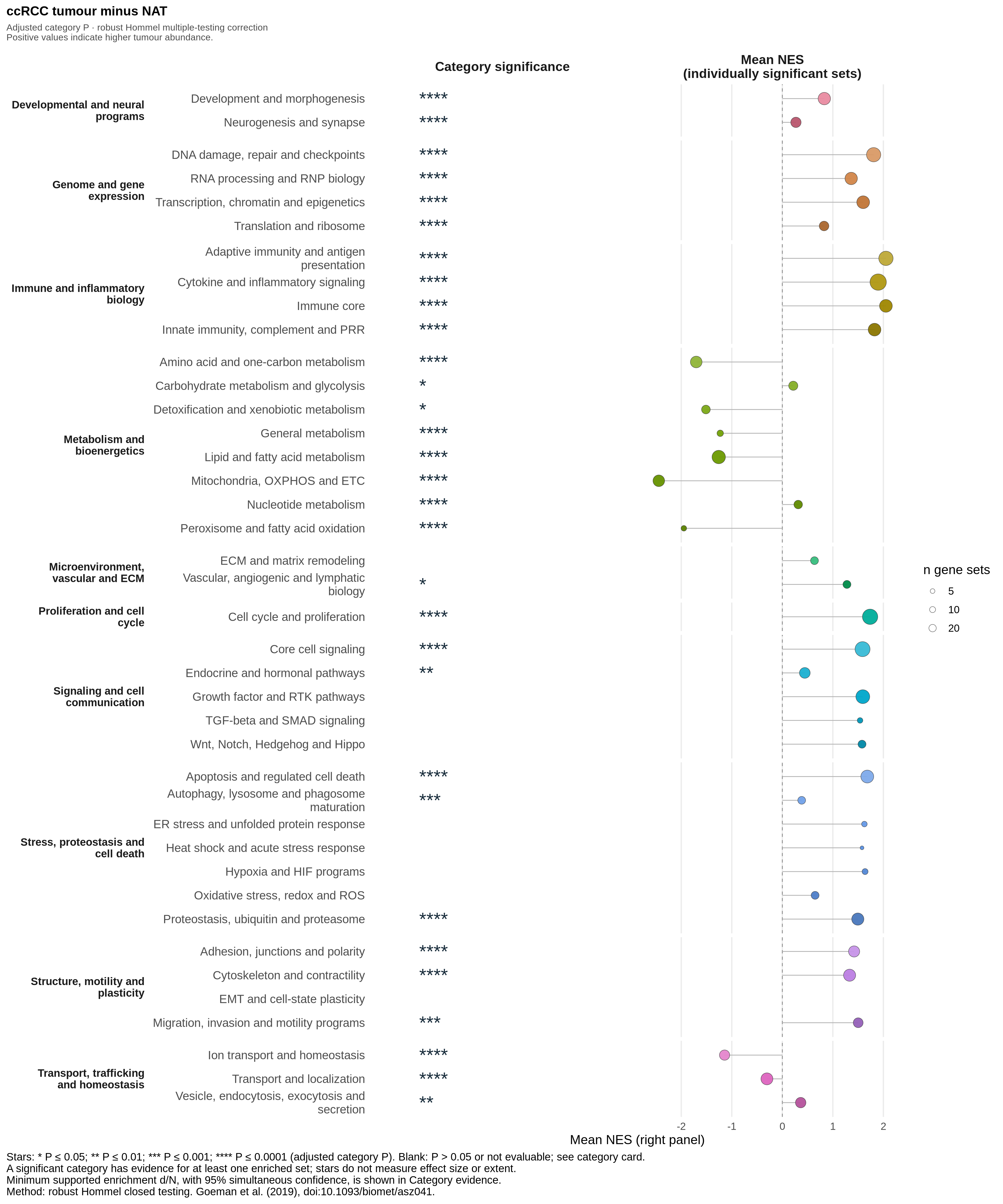
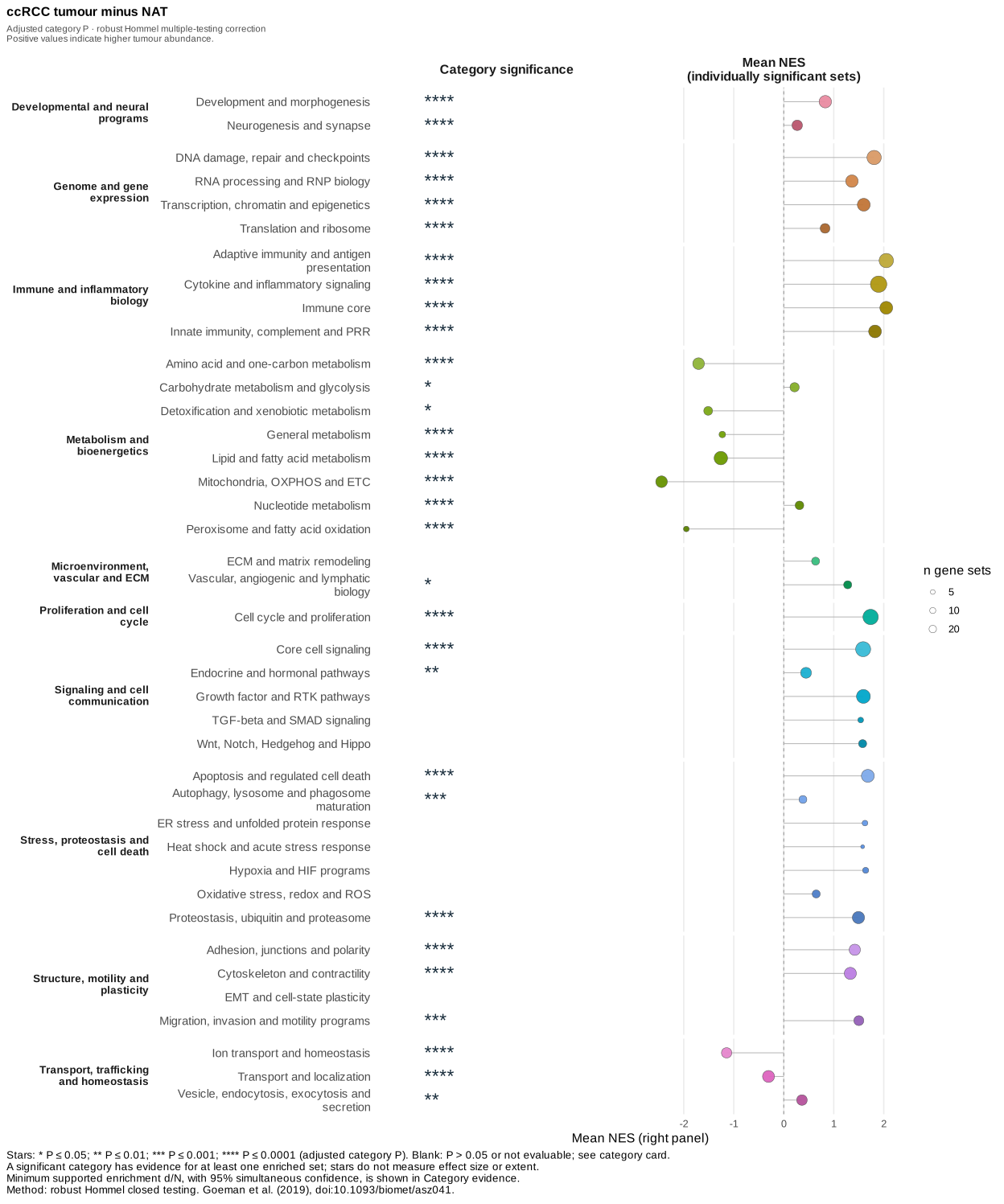
Each point shows descriptive mean NES of individually significant unique member gene sets (GSEA adjusted P ≤ 0.25); size is their count. Positive NES follows tumour minus adjacent tissue. Stars show Hommel-adjusted category P (one to four stars at ≤ 0.05, 0.01, 0.001 and 0.0001). Category significance is not inferred from mean NES or point size; blank means P > 0.05 or not evaluable. The 40 GOBP-C2 categories include 31 significant categories in this saved 80-pair example.

Full-size PNG, SVG, PDF, category results, plotted source and figure settings.

Optional upstream reconstruction

The prepared example bundle includes the DE table, not an executable reconstruction from raw mass spectra. A defensible upstream rebuild starts from an authorised processed abundance matrix and sample annotations from CPTAC/PDC. Reproduce the 80-pair selection, specify the paired limma design and preserve the protein-to-gene mapping, collision handling, filtering and missing-value decisions before exporting a complete ranked table. The supplied audit files identify the prepared input, but do not replace those source materials. This separate task is not run by the example preparer, and the guide does not claim a route from raw mass spectra.

What the five audit files document

The prepared project carries the primary DE table with five audit records: the matched-pair sample receipt, primary QC, data-quality summary, input provenance and the 80-pair list. They establish the input contract for this example. They do not substitute for access conditions, clinical context, sample processing information or an independent reanalysis of the source proteomics.

For another proteomic study, preserve the upstream mapping record, the number of measured features, the number retained after mapping and filtering, the duplicate policy, and missing-value handling with the prepared DE result. The Preparing DE inputs guide describes the general prepared-input contract.